Introduction
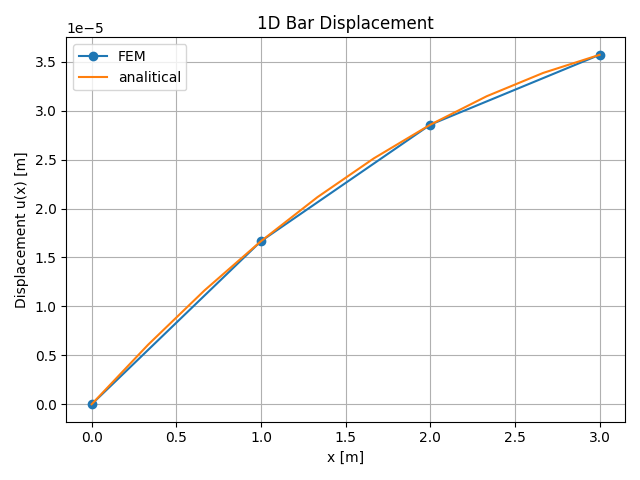
This example demonstrates the application of the Finite Element Method (FEM) to a 1D bar under axial tension. The bar is subjected to both a point load at its free end and a uniformly distributed load along its length. Using CALFEM for Python, we calculate the nodal displacements, reaction forces, and internal axial forces. This workflow illustrates the basic principles of FEM, including mesh generation, assembly of the global system, application of boundary conditions, and post-processing.
import numpy as np
import calfem.core as cfc
E = 210e9    # Young's modulus [Pa]
A = 0.001    # Cross-sectional area [m^2]
L = 3.0      # Length of the bar [m]
F = 1000.0   # Force at the right end [N]
q = 1000.0   # distributed load [N/m]
nel = 2
n_nodes = nel + 1
coords = np.linspace(0, L, n_nodes)
edof = np.array([[i, i+1] for i in range(1, nel+1)])
K = np.zeros((n_nodes, n_nodes))
f = np.zeros((n_nodes, 1))
for elx in range(nel):
    x1 = coords[elx]
    x2 = coords[elx + 1]
    Ke, fe = cfc.bar1e([x1, x2], [E, A], eq=[q])
    cfc.assem(edof[elx], K, Ke, f, fe)
f[-1, 0] = f[-1,0] + F
bc = np.array([1])
bc_val = np.array([0.0])
a, r = cfc.solveq(K, f, bc, bc_val)
for elx in range(nel):
    x1 = coords[elx]
    x2 = coords[elx + 1]
    ed = a[edof[elx] - 1]
    N = cfc.bar1s([x1, x2], [E, A], ed)
Material and Geometry
The bar has a defined Young’s modulus E, cross-sectional area A, and total length L. These material and geometric properties determine the stiffness and deformation behavior of the bar under load. In this example, the values chosen are typical for a structural steel bar.
Two types of loads are applied: a point load F at the rightmost node and a distributed load q along the bar. The distributed load is evenly applied across each finite element to simulate uniform stress along the bar.
Mesh Generation
The bar is divided into a number of finite elements nel. Each element connects two consecutive nodes, forming the element connectivity array edof. The number of nodes n_nodes is always one more than the number of elements. Node coordinates are evenly spaced along the bar length. This simple 1D mesh allows the bar to be modeled as a series of linear elements, each with its own stiffness and load contributions.
Assembly of the Global System
For each element, the element stiffness matrix Ke and the element load vector fe are calculated using CALFEM functions. The element contributions are then assembled into the global stiffness matrix K and global load vector f. After assembling the distributed loads, the point load at the free end is added directly to the corresponding node in the global load vector.
This assembly process combines the behavior of all elements into a single system of equations that represents the entire bar under the applied loads.
Boundary Conditions and Solution
Boundary conditions are applied to fix the left end of the bar, ensuring zero displacement at that node. The system of equations K * a = f is solved using the CALFEM solver, which returns the nodal displacements a and the reaction forces r at the constrained node. These results provide the primary solution for the bar’s deformation under the given loading conditions.