Introduction

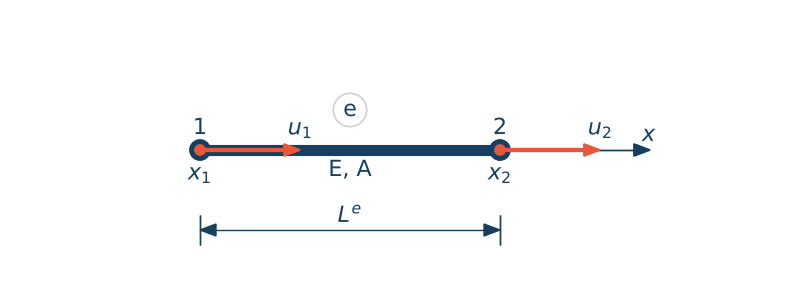
At the beginning, we briefly restate the 1D formulation that was introduced earlier, as it forms the basis for further development. We then extend this idea to truss structures in two dimensions. Conceptually, a truss element is nothing more than a bar that is arbitrarily oriented in space. However, this change in orientation introduces important geometric considerations. As illustrated in the figure below the above formulation is presented for a 1D bar (truss) finite element.

The element stiffnes matrix is defined as

$$\k = \cfrac{EA}{L^e}\begin{bmatrix}1 & -1 \\-1 & 1\end{bmatrix}$$

Although the element may be arbitrarily oriented in the global coordinate system, the formulation above is still expressed in the local coordinate system of the bar. This means that the displacement degrees of freedom are defined along the axis of the element (axial direction), independent of its orientation in space.

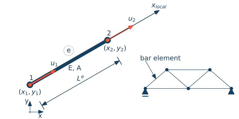
The key observation is that although the element exists in 2D, it still carries only axial forces. Therefore, its constitutive behavior remains identical to the 1D case — the only challenge is expressing this behavior in a global coordinate system. In other words, even for an inclined bar, the kinematic description remains one-dimensional, with displacements measured only along the element axis.

Consider a truss element defined by two nodes with coordinates:

• Node 1: $ (x_1, y_1) $
• Node 2: $ (x_2, y_2) $

The length of the element is:

$$L^e = \sqrt{(x_2 - x_1)^2 + (y_2 - y_1)^2}$$

To describe its orientation, we introduce direction cosines:

$$c = \frac{x_2 - x_1}{L^e}, \quad s = \frac{y_2 - y_1}{L^e}$$

These quantities represent the projection of the element axis onto the global coordinate axes. Unlike the 1D case, each node in 2D has two degrees of freedom: horizontal and vertical displacement.

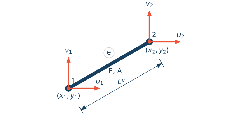
The physics does not change — only the coordinate system does. The element displacement vector is therefore:

$$\u_{global} =\begin{bmatrix}u_1 \\ v_1 \\ u_2 \\ v_2\end{bmatrix}$$

Transformation to Global Coordinates

We begin by denoting the stiffness matrix in the local coordinate system as:

$$\mathbf{k}_{\text{local}} = \frac{EA}{L} \begin{bmatrix} 1 & -1 \\ -1 & 1 \end{bmatrix}, \quad \u_{local} = \begin{bmatrix}1 \\-1\end{bmatrix}$$

To relate local quantities to global ones, we introduce a transformation matrix that projects global displacements onto the axis of the element:

$$\mathbf{T} = \begin{bmatrix} c & s & 0 & 0 \\ 0 & 0 & c & s \end{bmatrix}$$

This transformation is the key mechanism that introduces coupling between the $x$ and $y$ directions, even though the element itself only deforms axially. Using this matrix, the local displacement vector can be expressed in terms of global displacements as:

$$\mathbf{u}_{\text{local}} = \mathbf{T} \, \mathbf{u}_{\text{global}}$$

This transformation is the key mechanism that introduces coupling between the $x$and $y$ directions.

To obtain the stiffness matrix in global coordinates, we perform a coordinate transformation:

$$\mathbf{k}_{global} = \mathbf{T}^T \mathbf{k}_{\text{local}} \mathbf{T}$$

Carrying out this operation leads to the final expression:

$$\mathbf{k}_{global} = \frac{EA}{L^e} \begin{bmatrix} c^2 & cs & -c^2 & -cs \\ cs & s^2 & -cs & -s^2 \\ -c^2 & -cs & c^2 & cs \\ -cs & -s^2 & cs & s^2 \end{bmatrix}$$

This matrix captures both the material behavior and the geometric orientation of the element.

Generalization to 3D

The extension to three dimensions follows the same logic. Each node now has three degrees of freedom, and the element orientation is described by three direction cosines.

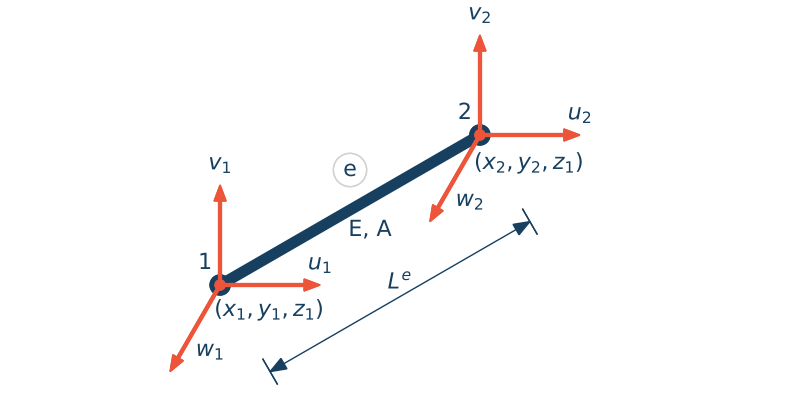
Although the size of the matrices increases, the structure of the formulation remains unchanged.

$$\mathbf{u}_{global} = \begin{bmatrix} u_1 \\ v_1 \\ w_1 \\ u_2 \\ v_2 \\ w_2 \end{bmatrix}$$

Let the element connect nodes:
• $(x_1, y_1, z_1) $
• $ (x_2, y_2, z_2) $

Then:

$$L^e = \sqrt{(x_2-x_1)^2 + (y_2-y_1)^2 + (z_2-z_1)^2}$$

Direction cosines:

$$l = \frac{x_2 - x_1}{L}, \quad m = \frac{y_2 - y_1}{L}, \quad n = \frac{z_2 - z_1}{L}$$

These define the orientation of the element in space. In analogy to the 2D case, we relate local (axial) displacements to global ones using a transformation matrix:

$$\mathbf{u}_{\text{local}} = \mathbf{T} \, \mathbf{u}_{\text{global}}$$

where:

$$\mathbf{T} = \begin{bmatrix} l & m & n & 0 & 0 & 0 \\ 0 & 0 & 0 & l & m & n \end{bmatrix}$$

This matrix projects global displacements onto the element axis. Transformation of the Stiffness Matrix. The global stiffness matrix is obtained using.

$$\mathbf{k}_{global} = \mathbf{T}^T \mathbf{k}_{\text{local}} \mathbf{T}$$

After carrying out the multiplication, we obtain:

$$\mathbf{k}_{global} = \frac{EA}{L^e} \begin{bmatrix} l^2 & lm & ln & -l^2 & -lm & -ln \\ lm & m^2 & mn & -lm & -m^2 & -mn \\ ln & mn & n^2 & -ln & -mn & -n^2 \\ -l^2 & -lm & -ln & l^2 & lm & ln \\ -lm & -m^2 & -mn & lm & m^2 & mn \\ -ln & -mn & -n^2 & ln & mn & n^2 \end{bmatrix}$$

Assumptions for Truss Elements

It is important to clearly state the assumptions underlying this formulation. Truss elements are based on several idealizations: members carry only axial forces, connections between elements are perfectly pinned, and loads are applied only at nodes.

Additionally, bending, shear, and torsional effects are neglected, and the analysis assumes small deformations. These simplifications make the formulation efficient but also limit its applicability.

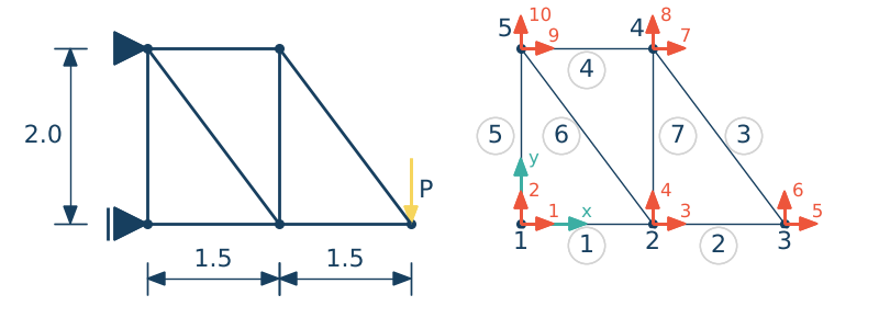
# Example