Beam Element

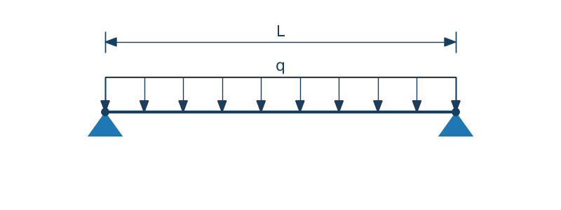
A cantilever beam is given, made of a material with stiffness $E$ and a cross-section whose moment of inertia is equal to $I$. The beam is subjected to a distributed load $q(x)$. The beam is fixed at the beginning.

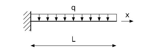
The differential equation describing the deflection of the beam axis is as follows

$$EI\cfrac{d^4 u(x)}{dx^4} = q(x)$$

The above equation is a fourth-order differential equation, so it must be supplemented with four boundary conditions
• deflection $u(x)$
• rotation angle $\cfrac{du}{dx}$
• bending moment $EI \cfrac{d^2u}{dx^2}$
• shear force $EI \cfrac{d^3u}{dx^3}$

Beam discretization

The size and character of the discretization are determined by the shape, loading, and material properties.

Equations describing the beam finite element

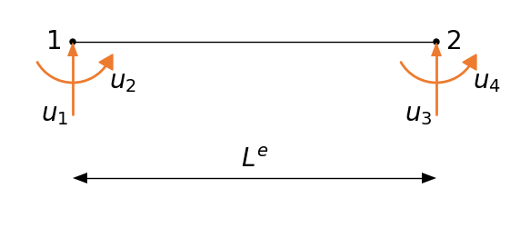
The approximate solution on a given element is sought for the following polynomial

$$u(x) \approx \sum_{i=1}^{4} u_iN_i$$

where $u_i$ are unknown parameters (displacements and rotation angles of a given node). The shape functions are chosen as:

$$N_1(x) = 1 - 3\left(\cfrac{x-x_1}{x_2-x_1}\right)^2 + 2\left(\cfrac{x-x_1}{x_2-x_1}\right)^3 \quad N_2(x) = (x-x_1)\left(1-\cfrac{x-x_1}{x_2-x_1}\right)^2$$ $$N_3(x) = 3\left(\cfrac{x-x_1}{x_2-x_1}\right)^2 -2\left(\cfrac{x-x_1}{x_2-x_1}\right)^3 \quad N_4(x) = (x-x_1)\left[\left(\cfrac{x-x_1}{x_2-x_1}\right)^2 - \cfrac{x-x_1}{x_2-x_1}\right]$$

These are Hermite polynomials. These functions have the property that their values and first derivatives at the ends of the interval are equal to 0 or 1. For example, the function $N_1(x)$

$$N_1(x_1) = 1, \quad N_1(x_2) = 0, \quad \cfrac{dN_1(x_1)}{dx} = 0, \quad \cfrac{dN_1(x_2)}{dx} = 0$$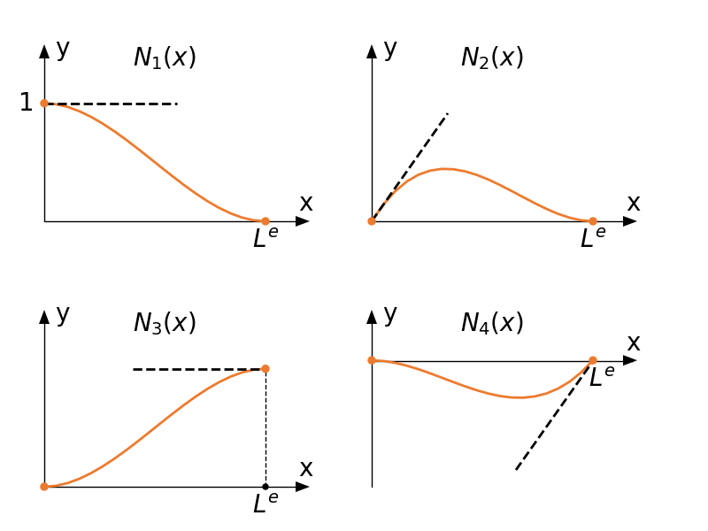

Let us write our approximate solution on the element in matrix form as before

$$u = \N\u, \quad \N = \begin{bmatrix} N_1 & N_2 & N_3 & N_4 \end{bmatrix}, \quad \u = \begin{bmatrix} u_1 & u_2 & u_3 & u_4 \end{bmatrix}^T$$

Substitute our approximate solution into the differential equation

$$R = EI\cfrac{d^4 \N\u}{dx^4} - q(x) \neq 0, \quad x \in \Omega$$

Multiply the residual by a weight equal to the function $u$ and integrate over the finite element. Set everything equal to zero (method of weighted residuals)

$$EI \int_{x_1}^{x_2} \N^T \cfrac{d^4 \N\u}{dx^4} dx - \int_{x_1}^{x_2} \N^T q dx = 0$$

Perform integration by parts twice for the first integral $\int f(x) \cdot g{'}(x) dx = f(x) \cdot g(x) - \int f{'}(x) \cdot g(x) dx$

$$EI \int_{x_1}^{x_2} \N^T \cfrac{d^4 \N\u}{dx^4} dx = -EI \int_{x_1}^{x_2} \cfrac{d\N^T}{dx} \cfrac{d^3 \N}{dx^3}dx \u+ EI \N^T \cfrac{d^3 \N}{dx^3}\u|_{x_1}^{x_2} =$$ $$EI \int_{x_1}^{x_2} \cfrac{d^2\N^T}{dx^2} \cfrac{d^2\N}{dx^2}dx \u + EI \N^T\cfrac{d^3 \N}{dx^3}\u|_{x_1}^{x_2} - EI \cfrac{d\N^T}{dx} \cfrac{d^2 \N}{dx^2}\u|_{x_1}^{x_2}$$

Introduce the following notation

$$Q_1^e = EI\cfrac{d^3 \N}{dx^3}\u|_{x_1}, \quad Q_2 = -EI\cfrac{d^2 \N}{dx^2}\u|_{x_1}, \quad Q_3 = -EI\cfrac{d^3 \N}{dx^3}\u|_{x_2}, \quad Q_4 = EI\cfrac{d^2 \N}{dx^2}\u|_{x_2}$$

After introducing the notation we obtain

$$EI \int_{x_1}^{x_2} \cfrac{d^2 \N^T}{dx^2} \cfrac{d^2\N}{dx^2}dx \u -\int_{x_1}^{x_2} \N^T q dx -\N^T Q_1 - \cfrac{d\N^T}{dx} Q_2 -\N^T Q_3 - \cfrac{d\N^T}{dx}Q_4 =0$$

Introduce further notation

$$\boldsymbol{k} = EI \int_{x_1}^{x_2} \cfrac{d^2 \N^T}{dx^2} \cfrac{d^2\N}{dx^2}dx, \quad \f = \int_{x_1}^{x_2} \N^T q dx, \quad \Q = \N^T Q_1 + \cfrac{d\N^T}{dx} Q_2 + \N^T Q_3 + \cfrac{d\N^T}{dx} Q_4$$

Using the above notation, our equations can be written as

$$\boldsymbol{k} _{4\times 4} \u_{4\times 1} = \f_{4\times 1} + \Q_{4\times 1}$$

Let us compute the first element of the stiffness matrix

$$k_{11} = EI \int_{x_1}^{x_2}\cfrac{d^2 N_1}{dx^2} \cfrac{d^2N_1}{dx^2}dx= \cfrac{12EI}{L^3}$$

Performing the above operations for all combinations of shape functions, we obtain

$$\boldsymbol{k} = \cfrac{2EI}{L^3} \begin{bmatrix} 6 & 3L & -6 & 3L\\ 3L & 2L^2 & -3L & L^2\\ -6 & -3L & 6 & -3L\\ 3L & L^2 & -3L & 2L^2\\ \end{bmatrix} \quad \f = \cfrac{qL}{12}\begin{bmatrix} 6\\ L\\ 6\\ -L\\ \end{bmatrix} \quad \Q = \begin{bmatrix} Q_1\\ Q_2\\ Q_3\\ Q_4\\ \end{bmatrix}$$

Assembly of finite elements

Combining finite elements into a single structure forming the beam requires satisfying conditions at each shared node. Consider two adjacent finite elements $e$ and $e+1$

• continuity conditions: continuity of deflection and continuity of rotation angles

$$\text{ugięcia} \quad u_3^e = u^{e+1}_1, \quad \text{obrót} \quad u_4^e = u_2^{e+1}$$

• equilibrium conditions of sectional forces (shear forces and bending moments)

$$\text{siła poprzeczna} \quad Q_3^e + Q^{e+1}_1 = 0, \quad \text{moment zginający} \quad Q_4^e = Q_2^{e+1} = 0$$

In the case where a concentrated force or bending moment is applied at a node, we have

$$\text{siła poprzeczna} \quad Q_3^e + Q^{e+1}_1 = P, \quad \text{moment zginający} \quad Q_4^e = Q_2^{e+1} = M$$

Introduce global numbering of nodal displacements

$$u_1^1 = U_1, u_2^1=U_2, \quad u_3^1 = u_1^2 = U_3, \quad u_4^1 = u_2^2 = U_4, ..., \quad u_4^N = U_{4(N+1)}$$

The next step is to construct the global stiffness matrix and the global load vector (analogous to the one-dimensional example)

$$\mathbf{K} \mathbf{U} = \mathbf{F}$$

where $\mathbf{F}$ is a vector that contains external loads and nodal loads. The above system of equations will contain $2(N+1)$ unknown nodal displacements, where $N$ denotes the number of elements. At each node we seek deflection and rotation angle.

Incorporation of boundary conditions

Similarly to the one-dimensional example, known deflections and rotation angles are substituted into the vector $\mathbf{U}$, while distributed and concentrated loads are included in the vector $\mathbf{F}$

---

# Example

---